Logistic Regression
A very popular concept in the world of machine learning operating in the supervised learning domain is the Logistic Regression. It is a linear classification algorithm finding its roots in the mid 19th century and really developed its pace for the scientific community in the late 1960ies.
Generally speaking, logistic regression aims to solve binary or dichotomous decision problems using the natural logarithm of an odds ratio and the logistic function. As the name reveals the algorithm displays some similarities to linear regression and tries to estimate in the same way as the latter a function generalising well on qualitative problems.
The article is structured as follows: First of all, some light will be shed on the basics and the algorithm itself as a concept. Thereafter, the underlying math of two distinct concepts, namely the Newton-Raphson-Method and the Gradient Descent, to run the algorithm are explained. In the following part, the two algorithms are implemented from scratch in Python and in addition to that, the sklearn library is used to apply the algorithm on some randomly generated data. After having explained the logic and use of the regularization parameter in Logistic Regression, it is described how to draw the decision boundary for this kind of classifier. The next section of the article treats the case of Logistic Regression with multiple classes, explains the concept and implements with Python. To close this deep dive into Logistic Regression, the properties of the algorithm are discussed.
The Algorithm
Logistic Regression is as mentioned in the introduction one of the most famous concepts in classification. In a nutshell, the algorithm takes one or more continuous or categorical variables as input variables and outputs a binary response.
Imagine a problem focuses on a data set out of the field of veterinary medicine. In the dataset, a record describes an animal, a dog or a cat, with his attributes (the independent variables or features) such as mean blood pressure, height, sleep time, etc. and the aim is to predict if the concerned animal is a cat or a dog – the dependent variable. If the animal is a cat the dependent variable is taking the value 1.0 and if not the variable value is 0.0.
In a binary classification problem, the decision between the two outcomes is based on probability: if the algorithm calculates a probability > 50 % for a data record the output variable is 1.0, otherwise ( it takes the value 0.0. At this point, it might be tempting to use just linear regression for the prediction in view of the fact that the output variable (the probability) is actually continuous and not categorical.
But first of all, linear regression doesn’t give out by default a value between 0 and 1 as it would be required for simple decision. Secondly, linear regression is due to the OLS-Method which is used to optimize the fit of the linear model prone to be sensitive to imbalanced data. In other words, linear regression is not the best way to approach such a problem without saying that this technique won’t work at all for challenges like that.
A more comfortable way of dealing with such a problem is Logistic Regression and it uses as you might derive from the name the linear regression model to optimize.
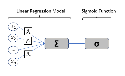
As shown on figure 1 above, the logistic regression algorithm can be divided in two distinct part: The first is a linear regression model where the features (in the example above, the mean blood pressure, sleep time, etc. of an animal in the dataset) are multiplicated with the respective weights and summed up to predict the dependent variable. In the second part, the so-called Sigmoid or logistic function squashes the value of the dependent variable into a space between 0 and 1 which represents the probability of the data record belonging to one of the two categories.
The central element of the Logistic Regression is the Sigmoid Function or also called the logistic function which you can see in the middle of the next figure.

Y=\begin{cases}1 & ,if\,animal\,is\,a\,cat\\0 & , if\,animal\,is\,a\,dog\end{cases}
In the following image slideshow the general steps are explained:
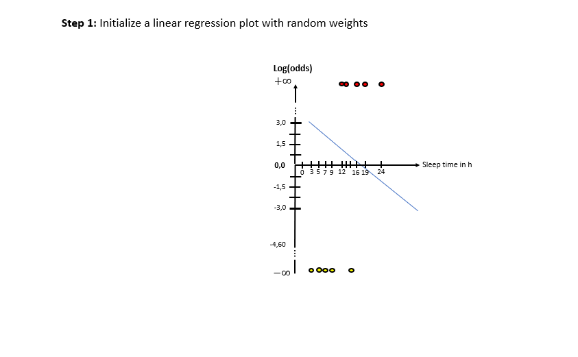
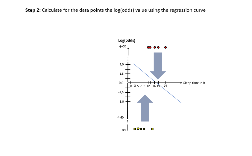
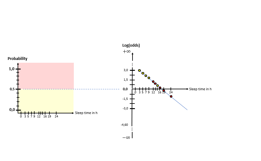
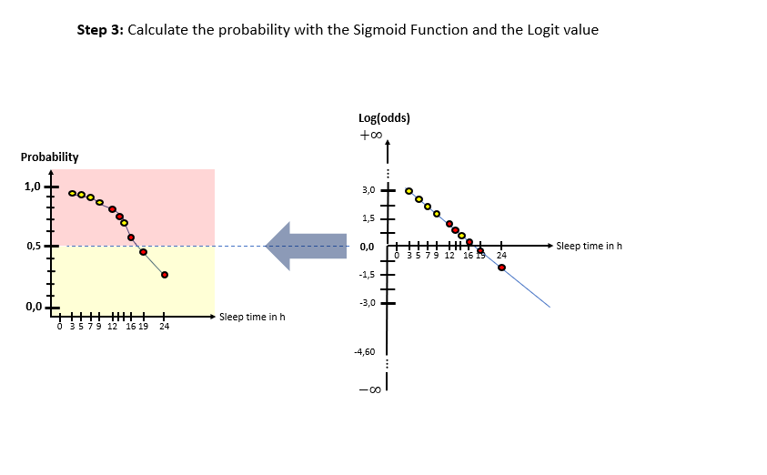
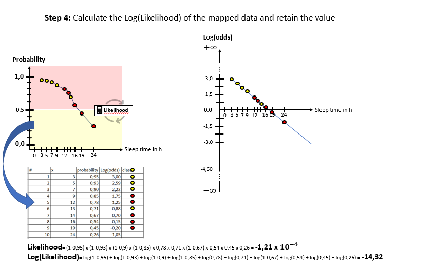
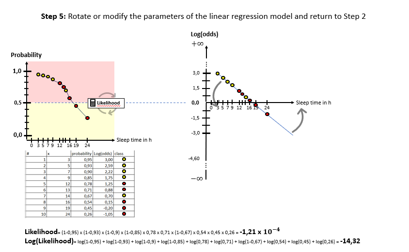
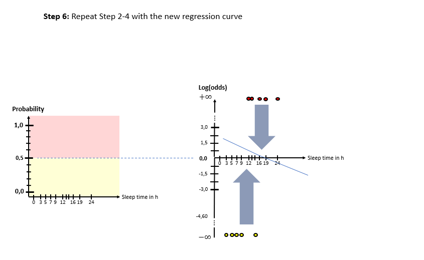
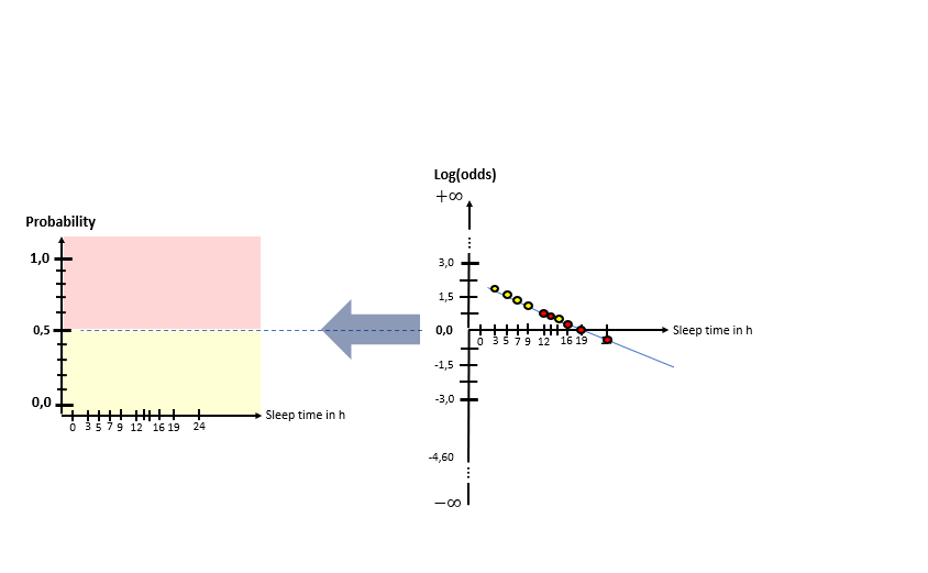
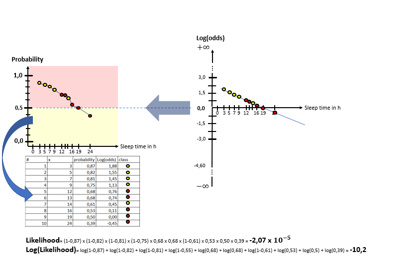
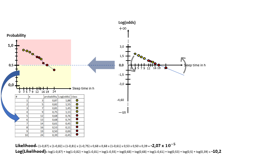
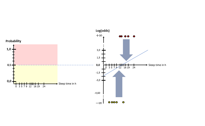
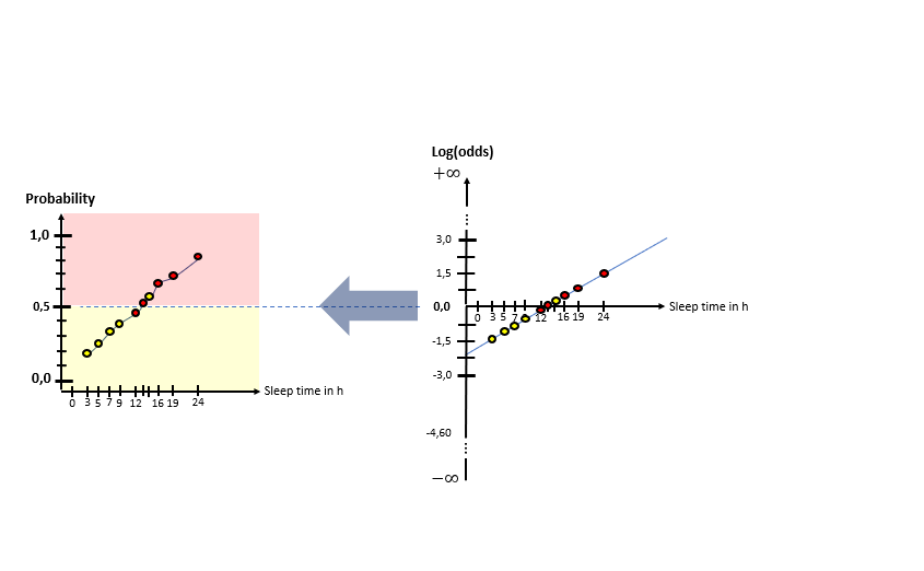
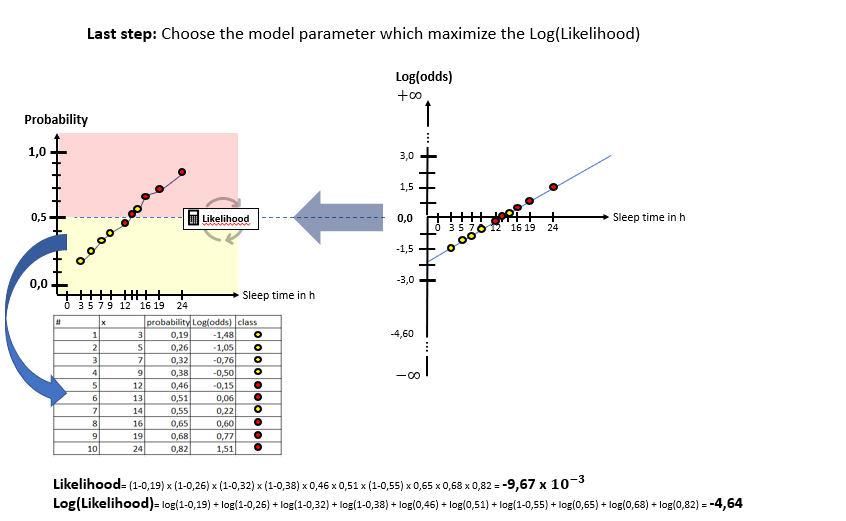
As one can see in the illustrations, there are two “spaces” involved: The X-Log(odds)-space and the X-Probability-space. The Odds-Ratio is really well explained by this source and can be described as the ration between the probability of an event happening to the probability of the counter-event happening. The regression model in the general form of lies in the “X-Log(odds)-Plane. For the respective animals the log(odds) value is calculated by means of the “sleep time in h” (X). With this result, the probability is calculated using the Sigmoid-Function. With the probabilities, a value for the Log-Likelihood Function is calculated. The latter represents the “quality measure” of the algorithm. The higher the value of the Log-Likelihood Function, the better the fit of the concerning regression curve in the X-Log(Odds)-space to the data. As one can the in the slide show, after having calculated the Log-Likelihood-value of the first (mostly randomly initialized) regression curve, the regression curve in the X-Log(Odds)-space is modified and the new Log-Likelihood-Value is calculated. This procedure is then repeated until the optimal parameters of the Linear Regression Model are found which maximize the Log-Likelihood function. After having finished this training phase of the algorithm to find the optimal parameters, the algorithm is ready to be used on real data.
Given a data point of a real data set, the algorithm takes its X-Values and calculates its probability value with respect to the calculated s in the training phase. The decision rule then is:
Y=\begin{cases}1 & ,if\,p(x)>0.5\\0 & , if\,p(x)\leq0.5\end{cases}As you can see, the fundamental goal of the training phase is to optimize the Log-Likelihood Function with the optimal parameters the linear regression model. There is more than one way to optimize Logistic Regression. The next section sheds a bit more light on the general mathematical relations and on the possible, mathematical paths to take, if you want to use Logistic Regression.
The Underlying Math
To provide a plain understanding of the concept, it is crucial to grasp first of all the basics. This is why in the first part of the current section the relation between the Sigmoid-Function and the Log(Odds) are explained. After that, the first way to find optimal parameters for the Logistic Regression is shown: The Maximum-Likelihood Method. The section closes with the mathematical exposition of the Gradient Descent algorithm to optimize the Logistic Regression parameters.
As mentioned further above, the Sigmoid or also-called Logistic function is the central element of the Logistic Regression.
The function looks as illustrated on figure x in the middle and has the form:
{I.,\,p(x)=\frac{1}{1+e^{(-\beta*x)}}}Some sources doesn’t use exactly this form and rather use this form:
{ \,\,p(x)=\frac{1}{1+e^{(-\beta*x)}}} {\,\,\,p(x)=\frac{1}{1+e^{(-\beta*x)}} * \frac{e^{(\beta*x)}}{e^{(\beta*x)}}} {II.\,\,p(x)=\frac{e^{(\beta*x)}}{1+e^{(\beta*x)}} }The relation between the Sigmoid function and the Logit or Log(Odds) can be derived as follows:
{ \,\,p(x)=\frac{1}{1+e^{(-\beta*x)}}} { \,\,p(x)*(1+e^{(-\beta*x)})=1} { \,\,p(x)+p(x)*e^{(-\beta*x)}=1} {\,\,p(x)*e^{(-\beta*x)}=1-p(x)} { \,\,e^{(-\beta*x)}=\frac{1-p(x)}{p(x)}} { \,\,e^{(\beta*x)}=\frac{p(x)}{1-p(x)}} { III.\,Logit=\beta*x=log(\frac{p(x)}{1-p(x)})}So as it is clearly visible, one can calculate the Log(Odds)-Ratio by means of the probability for a data record from the Sigmoid function and inversely, one can map the result of the Logit or Log(Odds)-Space to the probability space using the Sigmoid function.
Having this idea in mind, the next step is to focus on the Likelihood function which is the objective function to optimize.
It is possible to state that there are two possible events occurring either
\prod\limits_{s\,in\,y=1,\,i\,}p(x_{i}) \,\,\,\,\, or \prod\limits_{s\,in\,y=0,\,i\,}p(x_{i})The Likelihood-Function can be subsumed to:
L(\beta)=\prod\limits_{s\,in\,y=1,\,i\,}p(x_{i})\, * \prod\limits_{s\,in\,y=0,\,i\,}p(x_{i})\, L(\beta)=\prod\limits_{s,\,i\,}p(x_{i})^{y_{i}}\, * \prod\limits_{s,\,\,i\,}(1-p(x_{i}))^{(1-y_{i})}\,So for every data record where y=1, the Likelihood function exponentiates , the probability of the event y=1 happening, with 1 and exponentiates the counter-event with 0 which becomes just 1. Inversely, the same applies for the case y=0. So, if for a high number of data records the probability when y=1 is high and inversely if the probability when y=0 is low, the Likelihood-Function will put out a high value.
In practice, it is more convenient to work with the Log(Likelihood)-Function L . So:
L(\beta)=\sum_i^n y_{i}\,*\,log(p(x_{i}))\,+\,(1-y_{i})\,*\,log(1-p(x_{i}))and the same logic for the function to maximize holds as explained before.
As pointed out in the last section, the main goal of Logistic Regression is to maximize the Log(Likelihood)-Function. In other words, you want to minimize:
-L(\beta)=-\sum_i^n y_{i}\,*\,log(p(x_{i}))\,+\,(1-y_{i})\,*\,log(1-p(x_{i}))and this leads to the definition of the Loss-Function L:
V.\,\,\, L(\beta)=-\sum_i^n y_{i}\,*\,log(p(x_{i}))\,+\,(1-y_{i})\,*\,log(1-p(x_{i}))The minimization is executed by optimizing the parameters β, but because:
{ \,\,\,\,\,\,\,\,\,\,\,\,\,\,\,\,\,p(x)=\frac{1}{1+e^{(-\beta*x)}}}the Loss-Function is a transcendental equation meaning that it is not possible to find the optimal βs by an analytical approach.
The Algorithms presented in the following choose the way out in finding the optimal β by numerical means. The first one presented will be the Newton-Raphson-Method.
Logistic Regression with the Newton-Raphson-Method
As mentioned, the parameters \Large \beta optimizing the Loss-Function have to be found by numerical means. Nevertheless the condition for the optimal parameters \Large \beta holds as for every optimization problem:
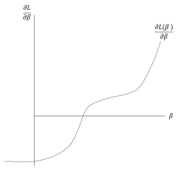
\frac{\delta L( \beta )}{\delta \beta }=0The Newton-Raphson-Method works as it is described graphically in the Slideshow xxx. The function \frac{\delta L( \beta )}{\delta \beta } , the first derivation of the Loss-Function, is shown in the \frac{\delta L( \beta )}{\delta \beta }-\beta-Space . The goal is to find a \beta where \frac{\delta L( \beta )}{\delta \beta }=0 through multiple iterations. At first random \beta s are initialized at point t. Then a tangent is drawn fitting the curve’s edge at \frac{\delta L( \beta_{t} )}{\delta \beta } . The tangent is hitting the abscissa at point \beta_{t+1} with the functional value \frac{\delta L( \beta_{t+1} )}{\delta \beta } . Hereafter another tangent is drawn fitting the edge of \frac{\delta L( \beta_{t+1} )}{\delta \beta } which subsequently leads to another point on the abscissa \beta_{t+2} . This procedure is then repeated until convergence of \frac{\delta L( \beta_{t+n} )}{\delta \beta }\approx0 . By this procedure, the optimal values for \beta -minimizing the Loss function \frac{\delta L( \beta )}{\delta \beta }=0\,\,- can be found.
To put it in a simple formula and to understand the relation, it is helpful to analyse the geometrics of this procedure:
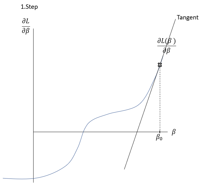
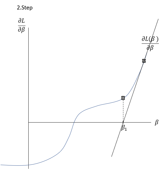
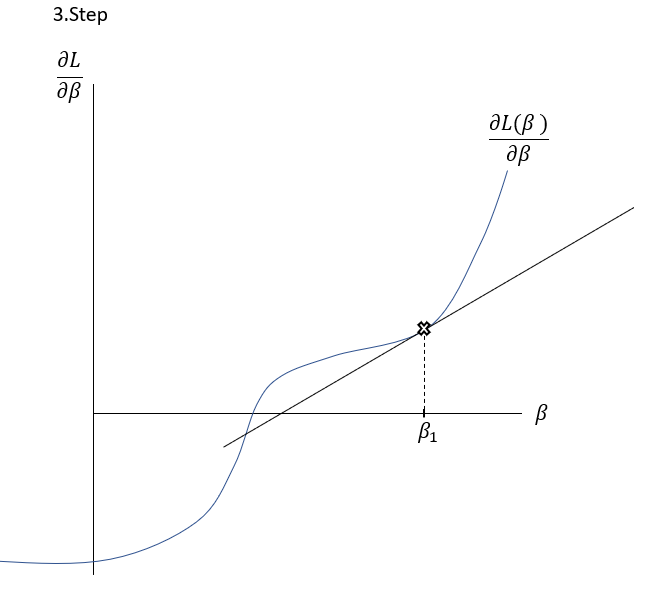
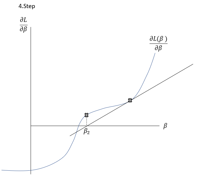
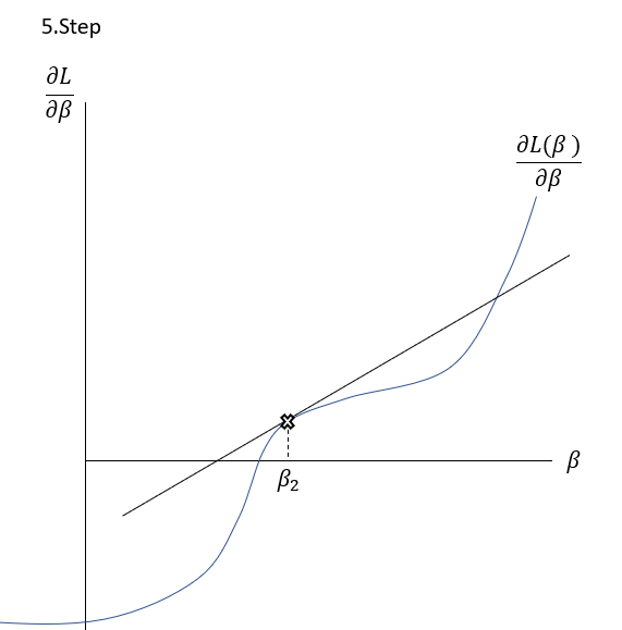
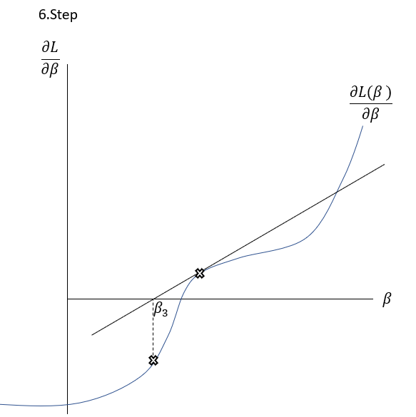
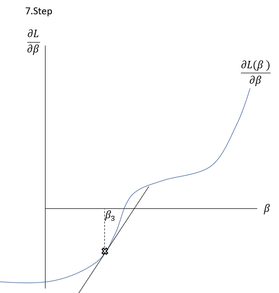
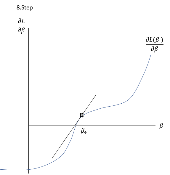
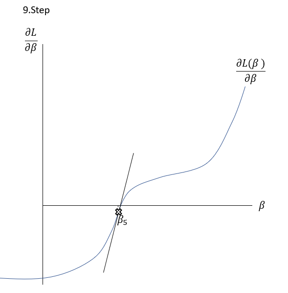
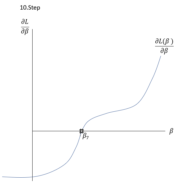

Having a look on the illustration above, the distance between and the new can be seen as the horizontal part of the gradient:
\frac{\delta^{2}L}{\delta^{2}\beta}(\beta)=\frac{\frac{\delta^{2}L}{\delta^{2}\beta}(\beta)}{\delta}Solving for \delta gives:
\delta=\frac{\frac{\delta L}{\delta\beta}(\beta)}{\frac{\delta^{2}L}{\delta^{2}\beta}(\beta}So, for getting the new parameter \beta_{t} , which is ideally more close to the functional value 0, the \beta_{t} has to be extended with \delta :
\beta_{t+1}=\beta_{t}-\frac{\frac{\delta L}{\delta\beta}(\beta)}{\frac{\delta^{2}L}{\delta^{2}\beta}(\beta}For calculating \beta_{t+1} , the derivations of the Loss-Function L(\beta) has to be calculated. But first of all, it is convenient to bring the equation V. in a more handy form:
L(\beta)=-\sum_i^n y_{i}\,*\,log(p(x_{i}))\,+\,(1-y_{i})\,*\,log(1-p(x_{i})) L(\beta)=-[\sum_i^n y_{i}\,*\,log(p(x_{i}))\,+log(1-p(x_{i}))-y_{i}*\,log(1-p(x_{i}))] L (\beta)=-[\sum_i^n y_{i}\,*\,\underbrace{log(\frac {p(x_{i})}{(1-p(x_{i}))})}_{Logit}\,+log(1-p(x_{i}))] L (\beta)=-[\sum_i^n (y_{i}\,*\,\beta\,*x_{i})\,+log(\underbrace{p(x_{i})}_{Sigmoid}\,*\, \frac{1}{e^{\beta*x}})] L (\beta)=-[\sum_i^n (y_{i}\,*\,\beta\,*x_{i})\,+log(\frac{1}{(1+e^{-\beta*x})}\,*\,\frac{1}{e^{\beta*x}})] L (\beta)=-[\sum_i^n (y_{i}\,*\,\beta\,*x_{i})\,+log(\frac{1}{1+e^{\beta*x}})] L (\beta)=-[\sum_i^n (y_{i}\,*\,\beta\,*x_{i})\,+log((1+e^{\beta*x})^{-1})] L (\beta)=-[\sum_i^n (y_{i}\,*\,\beta\,*x_{i})\,-log((1+e^{\beta*x}))]After this slight transformation, it is now possible to derive the two elements of \delta :
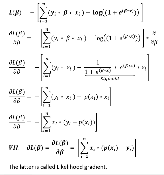
Determining \frac{\delta L}{\delta \beta} (\beta) :
Determining \frac{\delta^{2} L}{\delta^{2} \beta} (\beta) :
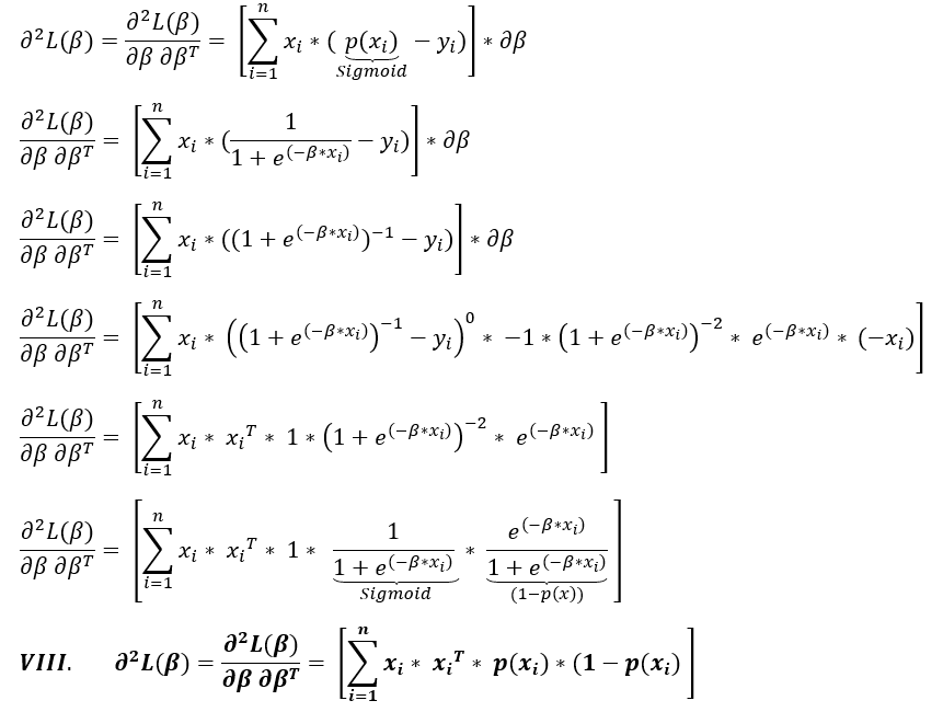
Bringing the equations VII. and VIII. together in the formula of Newton-Raphson to calculate the n^{th} iteration to approximate zero (equation VI.):

After having now understood the algorithm in depth, it can be subsumed under:
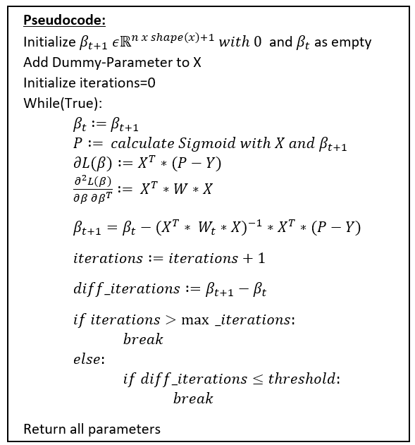
The results of this training phase can then be used to predict unknown real data. The Newton-Raphson is a very popular method to optimize the Logistic Regression Classifier for relatively small datasets. Because of the high computational cost of the calculation of the Likelihood gradient including the Hessian, it is not the best choice for large datasets.
The next algorithm to fit Logistic Regression takes either an iterative approach and is called Gradient Descent.
The results of this training phase can then be used to predict unknown real data. The Newton-Raphson is a very popular method to optimize the Logistic Regression Classifier for relatively small datasets. Because of the high computational cost of the calculation of the Likelihood gradient including the Hessian, it is not the best choice for large datasets.
Logistic Regression with the Gradient-Descent Method
The Gradient Optimization Algorithm to fit the Logistic Regression parameters starts also with the Loss-Function V.:
L(\beta)=-\sum_i^n y_{i}\,*\,log(p(x_{i}))\,+\,(1-y_{i})\,*\,log(1-p(x_{i}))The Sigmoid function which for now was defined as the probability p(x_{i} can also be defined as:
\large \sigma(z)=\frac{1}{e^{-z}}, where\,z=\beta\,*\,x_{i}The relation between the functions can be described as follows:

The goal is to derive \frac{\delta L(a,y)} {\delta z} to find the optimal parameters \beta.
But as the illustration expresses quite well, it is not possible to differentiate the Loss-Function L(a,y) directly with respect to \beta . This is when the so-called Back-Propagation which is equally used in Neural Networks into play. The derivation is split up by the chain-rule:
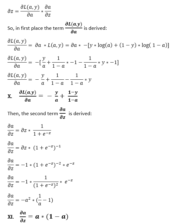

The equation XII. is actually the Likelihood-Gradient from the equation VII., we derived in the section “Logistic Regression with Newton-Raphson”. The iterative change of \beta can be described by means of \delta z as:
XIV.\,\, \delta \beta=\frac{\delta L(a,y)}{\delta \beta}=x^{T}\,*\,\delta zFor updating the weights\beta ,
including the intercept, the Likelihood-Gradient multiplicated with a learning rate is subtracted from the current weights:
\beta_{t+1}\,:=\,\beta_{t}-\underbrace{\alpha}_{Learningrate}\,*\,\delta \betaFor the training phase, the following algorithm is executed:
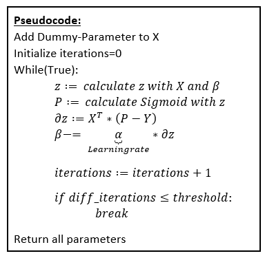
After this training phase, the fitted parameters can be used to predict unknown data.
The prediction-method of the algorithm then implements a simple if-clause which sets for each data record by means of the respective calculated probability-value (Sigmoid-value) for values for probabilities above 0,5 a 1.0 and for probability-values below or equal 0,5 a 0.0.
It should be noticed that this two algorithm are just two of many algorithm which can be used to fit a Logistic Regression to data sets. But the present explanation covers the two main algorithm used to train the model.
In the next section, the two optimization algorithm will be implemented in Python, on the one hand from Scratch and on the other hand by the famous sklearn-library.
In the next three sections of the article, the algorithm will be implemented with the Newton-Raphson-Method as well as the Gradient Descent from scratch. Then it will be shown how an implementation with the sklearn library works out.
Implementation from Scratch in Python: The Newton-Raphson-Method
Implementation from Scratch in Python: The Gradient-Method-Method
Implementation with sklearn in Python
Regularization
Looking at the sklearn library, the logistic function class takes beside the solver where it is possible to decide about the optimization algorithm used for the training phase and other parameters also the arguments “penalty” and “C”. It is the so-called “Regularization”-Parameter. Regularization can be seen as a way to penalize overfitting and assure the generalization of the algorithm on unseen data. In short: Overfitting occurs if the parameters of an algorithm are too tuned on the training data what causes partly poor performance on unknown test or real data and regularization limits the effect of overfitting.
Mathematically, a regularization term is added to the cost function like for example in L2-Regularization:
L(\beta)=- \sum_i^n y_{i}\,*\,log(p(x_{i}))\,+\,(1-y_{i})\,*\,log(1-p(x_{i}))+\underbrace{\frac{\lambda}{2}\,*\,||\beta||^{2}}_{L2-Penalization-Term}This term contains the complexity parameter that controls the amount of shrinkage. When minimizing the cost function, the larger the second term of the equation, the smaller the first term. In this logic, while minimizing function there’s a trade off between fitting the training data and the parameters \beta being small.
With the argument „penalty“ of the sklearn-library, it is possible to choose the penalization method and the „C“-parameter is the inverse of \lambda . So, the smaller \lambda is chosen, the higher is the penalization.
Closing this section of the article, it is worth to mention that also the regularization parameter of an algorithm such as Logistic Regression has to be chosen in light of the “No free lunch-Theorem” wisely and individually depending on the underlying data.
How to plot the decision boundary?
To fit the algorithm to the underlying data and using it on test or real data is the most principal thing to understand in Logistic Regression. But also the way to visualize the data and the decision boundary of the algorithm plays a major role to efficiently transmit the result of the algorithm to other stakeholder in your business.
For the 2-D Space, the decision boundary can be subsumed to:
f(x)=\beta_{0}+\beta_{1}\,*\,x_{1}+\beta_{2}\,*\,x_{2} 0=\beta_{0}+\beta_{1}\,*\,x_{1}+\beta_{2}\,*\,x_{2} \beta_{2}\,*\,x_{2}=-\beta_{0}-\beta_{1}\,*\,x_{1} x_{2}=-\frac{\beta_{0}-\beta_{1}\,*\,x_{1}}{\beta_{2}}To see how a decision boundary is implemented in a programming language, it is useful to take a glance on the implementation section of this article.
Logistic Regression for multiclass problems
Originally Logistic Regression is a binary classifier. But it can also be used to solve multiclass decision problems. There are multiple ways to tackle this kind of problems, but the main two are the one-vs-all and the one-vs-one method.
In both method the multiclass model is build based on multiple binary Logistic Regression classifier.
In the on-vs-all or also-called one-vs-rest method, if there are C classes, C binary classifiers are trained for each class as it is observable in the figure.

Properties to know of Logistic Regression
In this part of the article, some light will be shed on the properties of the algorithm leading to advantages as well as disadvantages which makes it so popular in the world of machine learning.
First of all Logistic Regression is a very simple algorithm on multiple levels: With the necessary background, it is quite simple to implement and the results are easy to interpret, what represent a great advantage when communicating them to public. In addition to that, the computational resources needed to calculate the algorithm is in comparison with decision trees or deep learning quite low, even if one should pay attention to the optimizer to use for which size of data. Underlining this idea of simplicity, overfitting can be straightforward inhibited by adding regularization to the algorithm.
But beside the big advantages, the algorithm exhibits also its downsides. Basically, Logistic Regression suffers from the same problems as linear regression. For example, the performance of the algorithm reduces or in extreme cases doesn’t work if the data isn’t precleaned (outliers, missing data , etc.) or if the independent variables exhibit strong collinearity. This linear relationship which isn’t desirable between the independent variables should be obligatory be present between the independent and the dependent variable to obtain reliable results with this linear classifier. In addition to that, the algorithm needs to be fed with relevant independent variables otherwise it fails to perform correctly. From this point of view, before using the algorithm, relevant features has to be discovered extracted and sometimes engineered of the underlying data. Another disadvantage of the concept lies in the fast that Logistic Regression can’t handle more complex or non-linear problems and is limited to data with linear relationship. Moreover, the concepts tends sometimes to overfit and therefore the user has to be careful in tuning the regularization parameter so that the concept generalizes well on test or real data.
Sources
- Ashishverma (2016): Logistic Regression – Part 2. Online verfügbar unter https://whyml.wordpress.com/tag/logistic-regression/.
- Brixius, Nathan (2016): The Logit and Sigmoid Functions. Hg. v. Nathan Brixius. Online verfügbar unter https://nathanbrixius.wordpress.com/2016/06/04/functions-i-have-known-logit-and-sigmoid/.
- Brownlee, Jason (2016): Logistic Regression for Machine Learning. Hg. v.
- MachineLearningMastery.com. Online verfügbar unter https://machinelearningmastery.com/logistic-regression-for-machine-learning/.
- Chatterjee, Sharmistha (2019): A Comprehensive Study of Linear vs Logistic Regression to refresh the Basics. Online verfügbar unter https://towardsdatascience.com/a-comprehensive-study-of-linear-vs-logistic-regression-to-refresh-the-basics-7e526c1d3ebe.
- CodeEmporium (2018): Logistic Regression – THE MATH YOU SHOULD KNOW! Hg. v. CodeEmporium-on-Youtube. Online verfügbar unter https://www.youtube.com/watch?v=YMJtsYIp4kg.
- Cramer, J S (2002): The Origins of Logistic Regression. Discussion Paper. Tinbergen Institute; University of Amsterdam, Amsterdam. Faculty of Economic and Econometrics.
- Goodfellow, Ian; Bengio, Yoshua; Courville, Aaron (2016): Deep Learning. Hg. v. MIT Press. Online verfügbar unter http://www.deeplearningbook.org, zuletzt geprüft am 20.06.2019.
- Hastie, Trevor; Tibshirani, Robert; Friedman, Jerome H. (2017): The elements of statistical learning. Data mining, inference, and prediction. Second edition, corrected at 12th printing 2017. New York, NY: Springer (Springer series in statistics).
- James, Gareth; Witten, Daniela; Hastie, Trevor; Tibshirani, Robert (2017): An introduction to statistical learning. With applications in R. Corrected at 8th printing. New York, Heidelberg, Dordrecht, London: Springer (Springer texts in statistics).
- Jing, Hong (2019): Why Linear Regression is not suitable for Classification. Hg. v. medium.com. Online verfügbar unter https://towardsdatascience.com/why-linear-regression-is-not-suitable-for-binary-classification-c64457be8e28.
- Kleinbaum, David G.; Klein, Mitchel; Pryor, Erica Rihl (2002): Logistic regression. A self-learning text. 2nd ed. New York: Springer (Statistics for biology and health).
- Marsland, Stephen (2015): Machine learning. An algorithmic perspective. Second edition. Boca Raton, FL: CRC Press (Chapman & Hall / CRC machine learning & pattern recognition series).
- Ng, Andrew (na): Exercise 5: Regularization. Hg. v. Stanford University. Online verfügbar unter http://openclassroom.stanford.edu/MainFolder/DocumentPage.php?course=MachineLearning&doc=exercises/ex5/ex5.html.
- Ng, Andrew: Lecture 6.5 — Logistic Regression | Simplified Cost Function And Gradient Descent — [ Andrew Ng]. Online verfügbar unter https://www.youtube.com/watch?v=TTdcc21Ko9A.
- Ng, Andrew (2016): Lecture 6.7 — Logistic Regression | MultiClass Classification OneVsAll — [Andrew Ng]. Hg. v. Artificial Intelligence – All in One. Online verfügbar unter https://www.youtube.com/watch?v=-EIfb6vFJzc.
- Paul, Michael (2018): Multiclass and Multi-label Classification. University of Colorado Boulder, Colorado Boulder.
- Pellarolo, Martín (2018): Logistic Regression from scratch in Python. Hg. v. medium.com. Online verfügbar unter https://medium.com/@martinpella/logistic-regression-from-scratch-in-python-124c5636b8ac.
- Pfeifer, Ralf (2005): Animation of Newton’s method. Hg. v. wikimedia.org. Online verfügbar unter https://commons.wikimedia.org/wiki/File:NewtonIteration_Ani.gif.
- Robinson, Nick (2018): The Disadvantages of Logistic Regression. Hg. v. theclassroom.com. Online verfügbar unter https://www.theclassroom.com/disadvantages-logistic-regression-8574447.html.
- scikit-learn.org (na): sklearn.linear_model.LogisticRegression. Online verfügbar unter https://scikit-learn.org/stable/modules/generated/sklearn.linear_model.LogisticRegression.html.
- Species, Iris (2016): Logistic Regression Classifier – Gradient Descent. Hg. v. Kaggle.com. Online verfügbar unter https://www.kaggle.com/msondkar/logistic-regression-classifier-gradient-descent.
- Sphinx-Gallery: Logistic function. Hg. v. scikit-learn.org. Online verfügbar unter https://scikit-learn.org/stable/auto_examples/linear_model/plot_logistic.html.
- Starner, Josh (2018): Logistic Regression Details Pt 2: Maximum Likelihood. Hg. v. Statquest-on-Youtube. Online verfügbar unter https://www.youtube.com/watch?v=BfKanl1aSG0&t=188s.

