Ensemble Learning

Every average person faces multiple time in his life important decisions such as for example the purchase of a house or a car. Within the decision process, it is quite unlikely that the person in question purchases without any prior knowledge the first good he encounters, which meets his requirements. He would search in the web for useful hints and comparable offers. He would ask friends, colleagues and other experts he know for help and their opinion to come eventually to a decision that combines all his information he gathered within the decision process. In essence, the person in question would build a committee and would decide in favor of the option which has been voted for of the most. The concept of Ensemble Learning follows the same idea: On a given data set multiple classifiers or regressors are built and the combined results of all members of that expert committee form the prediction for
the given problem.

Ensemble Learning Deep Dive

To analyze the method a bit deeper, it is useful to develop a clear definition of an ensemble learning model:

An ensemble learning model can be described as a powerful and popular meta-machine learning model combining the individual estimations of several, distinct,
simple machine learning models in order to output an estimation outperforming every single one of them and using the strengths of each member of the this
decision committee. In general, an ensemble model has a determined set of building blocks:

Training set: consists of a matrix $X^{nxm}$ , containing the training input attributes $x_{i}$ , and a vector $Y^{nx1}$ , containing the target class labels or continuous values $y_{i}$ depending on the machine learning task (classification or regression).
Base inducer: is the algorithm producing the machine learning models from the n tuples ( $x_{i}$ , $y_{i}$ ) representing the generalized relationship between the input and the target variable.
Diversity generator: this building block assumes the task to generate independent classifiers to ensure a good performance of the ensembling model.
Combiner: to output an aggregated estimate. This component combines the results of the individual models.

These building blocks are responsible for a good functioning and are present in every Ensemble Model. It is possible to distinguish independent ensemble from dependent ones.

For building the former, several datasets are drawn (overlapping or exclusive) from the underlying data to train the individual models upon the respective sub-datasets. In the second step, the resulting outputs are then combined in a predefined way.

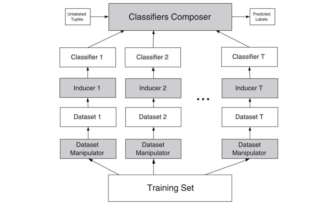
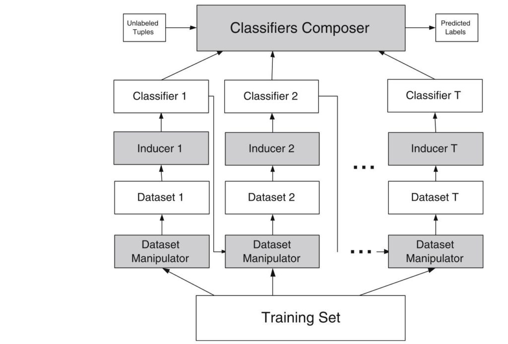
In a dependent ensemble model, on the other side, the individual models aren’t constructed in parallel like in in bagging, but in an incremental approach. There two categories of dependent ensembles:

On the one hand, there are dependent models using incremental batch learning. Here, the individual models are built one after another and each model uses the output of the prior modelin relation with the training set to output the next estimation. The model which is built at the last iteration is used to estimate the final prediction.

On the other hand, dependent ensembles can also be built using model-guided instance selection. Within this method, at the beginning equal weights are assigned to each of the training tuples what means that the individual model built upon the data focuses on each instance of the data equally. Then i an incremental fashion, the individual models change these weights at the respective iteration getting following models to focus stronger on parts o the data which haven’t been predicted well so far. A well-known representative of model-guided instance selection is boosting. The schema of the procedure of the dependent ensembles is illustrated in figure 2.

But what are the prerequisites for a good ensemble model?

First of all, it is necessary to clarify that an ensemble model have to be itself accurate and diverse to output better results than its individual components. In this context, an accurate model is one obtaining an error rate which is better than random guessing when being confronted with unseen input data. To consider two individual models being diverse, they have to make different errors on new data. If the individual models aren’t diverse, the idea of letting a committee of experts decide over the final output for a given input $x_{i}$ doesn’t make sense anymore: If model 1 is wrong, model 2 and model 3 are also wrong. But if the individual models are diverse (e.g. model 1 is wrong, model 2 and model 3 are correct), within the chosen way of combining the individual outputs, the probability is high that the correct output will be chosen.

To put it in other words: if the error rate of m individual models are all below 0.5 (so they deliver individually better results than random guessing) and if the error rates are uncorrelated, the probability that the majority vote of the ensemble model (the result of half or more of the individual models) is wrong could described as the area under the curve of a binomial distribution, where more than $\frac{m}{2}$ models are wrong.

Considering the case where $m=21$ and each of these models attains an error rate of 0.3. The probability that 11 or mre models are guessing simultaneously wrong is 2.6 %, which is much less than the erorr rate of each individual model.

The previous explanations described the prerequisites of a good ensemble model and their impact on the performance of it with respect to the performance of its individual components.

But there are three even more precise reasons why an ensemble can work better than a single model:

In literature, it is possible to distinguish statistical, computational and representational reasons.

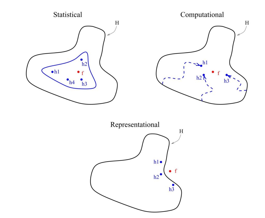
Statistical reasons: When training an algorithm on a given dataset, the model searches the optimal solution for the given problem in the of hypothesis H. Given insufficient data (e.g. the given data to learn is in relation to the hypothesis space to small), many different individual models with their respective hypothesis $h_{x}$ (see figure 3, top left) can be found with a comparable accuracy. But even with a very clever and well-thought model setting, there is always an uncertainty concerning the output of an individual model being wrong. To reduce this risk of choosing the wrong model as final prediction, ensemble models take the average result of the m trained models. In Figure 3, an extract of Dietterich, Thomas (2000)’s work, on the top left, the fou hypothesis of their respective models in H and the correct hypothesis f are shown. By averaging { $h_{1},h_{2},h_{3},h_{4}$ }, it is possible to approximate the true hypothesis f satisfactorily.
Computational reasons:
Depending on the specification and the learning concept of the given algorithm, it is possible that the latter finds a local optimum while learning instead of proceeding to the global optimum (e.g. decision trees or neural networks). Choosing now one of the hypothesis resulting from these models mentioned above, the chosen hypothesis reflects instead of the true hypothesis f a local optima. To provide a better approximation for f, the distinct hypothesis attaining the local optimas are averaged within an ensemble model (Figure 3, top right).
Representational Reasons
Considering a non-linear learning problem, whose true hypothesis value is not situated within the hypothesis space H covered by the different individual models (Figure 3, bottom), it is difficult to approximate the true hypothesis f using the output of a linear learning model. So, it may be possible to approximate $f \notin H$ by weighting or averaging the hypothesis of the different hypothesis $\in H$ (see Figure 3, bottom).

Having now a solid understanding of functioning and the performance of ensemble models, it is also useful to discuss the most important mechanisms to combine different, individual models within ensemble modeling.

There is for example the possibility to weigh the different estimates concerning their estimated or training accuracy (e.g. weighted averaging). Another popular approach would be majority voting. This method is used for example when the target variable of the prediction problem is categorical. There are other possibilities to combine the individual results, but this article does not undertake further investigations for other options, because the two options mentioned before combined with cross-validation are the most popular ones.

In the following, two of the most well-known ensembling methods are described more in detail.

Bagging

One of the most well-known independent ensemble modeling methods is the so-called bootstrap-aggregating or bagging. As the name uncovers, the method consists of a bootstrap and a aggregation step. In Figure 4, James et al.(2017) subsume the general process of this approach.

Within the bootstrap process, m (or in the figure: B) distinct sub-datasets are sampled with replacement in parallel. So, it is possible that each instance of S (or in the figure: Z) appears more than once or not at all. Thereby, each instance can be drawn with equal probability. The m (sub-)datasets are then used to train m preferably unstable learner (such as e.g. decision trees) $\hat{f}_{*i}(x)$ , building the committee of the ensemble model. For using the ensemble model on unseen data, the new datapoints are provided as input to the m learner and an average or a majority vote is established to obtain the final prediction:

\hat{f}_{avg}(x)=\frac{1}{m}*\sum_{i=1}^{m} \, \hat{f}_{*i}(x)

The ensemble improves in general the accuracy compared to the performance of the individual models. The method works (empirically proven) quite well with instable learner such as decision tre, but obtains also good performance with regression settings. In combination with stable learning methods there is no improvement of performance.

To estimate the performance of the model in terms of error rate, the so-called out-of-bag (OOB) observations are used to test the performance of the model. Each of the individual models, forming eventually the ensemble committee, uses in average $\frac{2}{3}$ of all observations in the training process. The remaining $\frac{1}{3}$ observations are the mentioned OOB observations. To obtain an estimate for the $i^{th}$ observation of the whole training set, all models of the ensemble are used for its prediction, for which the observation in question was an OOB observation. For the $i^{th}$ observation, there should be around $\frac{m}{3}$ models available for which the observation was an OOB observation. The OOB error yields quite valid results and can be seen as an good approximation of the test error for the bagged model.

One of the main virtues of bagging is the fact, that it helps to reduce variance of instable machine learning models or other weak learners and helps to overcome overfitting to improve the generalization performance. One of the major limitations of bagging arises from a statistical point of view in combination with decision trees: The trees tend to split data with more or less dominant input features in the same way and therefore the trees suffer in part from (strong) correlation, what can lead to a lower performance of the bagging technique.

Random Forest

Considering a bagged model built upon individual decision tree models, there is one major limitation, which has already been briefly mentioned in the section concerning the bagging approach: Within the tree building process, the respective inducer splits the respective remaining part of the original dataset at each stage in more homogenous parts to obtain eventually pure leaves concerning the class label or the prediction value. If the original dataset contains one (or more) strong predictor variable(s), there is a high probability that these predictors occur also in the subdatasets following a similar distribution as the original dataset. The distinct inducers calculate from the beginning on equally high scores for the different predictors leading to a similar splitting behavior. In this way, the structure of the individual trees can be highly correlated.

The main advantage of ensembling low biased, but highly volatile models such as decision trees lies in the reduction of their variance to find the best approximation for the true hypothesis. Averaging the results of the individual, highly correlated tree models does not reduce the variance as much as averaging the individual hypothesis of uncorrelated trees. To put it in a more formal form:

An average of m i.i.d. random variables has a variance of

\bar{\sigma}^{2}=\frac{1}{m}*\sigma^{2}

when these random variables are not independent, there exists a correlation $\rho$ and the variance could be defined as:

\bar{\sigma}^{2}=\rho * \sigma^{2}+\frac{1-\rho}{m}*\sigma^{2}

So, if $\rho=0$ , the term turns out to be $\frac{1}{m}*\sigma^{2}$ , the variance of an i.i.d. random variable. Keeping this in mind, it is easy to see that averaging m individual, correlated trees leads to approximately the same performance as the hypothesis of a single individual tree. Obviously the question arises how to overcome this difficulty.

The Random Forest model (RF) uses a clever tweak to solve the issue for obtaining competitive results. The idea behind RF is to reduce the correlation $\rho$ between the individual trees in order to reduce the variance of the bagging process without increasing the variance $\sigma^{2}$ too much. To reduce the correlation between the individual trees, after having terminated the bootstrapping process, the inducing process undergoes a slight change:

After having drawn m subdatasets throughout the bootstrapping process, the individual sets are provided to the m inducers. But instead of considering each of the p attributes for each split within the inducing process, the inducer draws randomly for each split $p_{s} \leq p$ of the input attributes which can be considered for the respective split. In this way, m uncorrelated trees can be obtained and the power of bagging can be unfolded. Setting $p_{s}=p$ would result in the normal bagging process without any adaption.

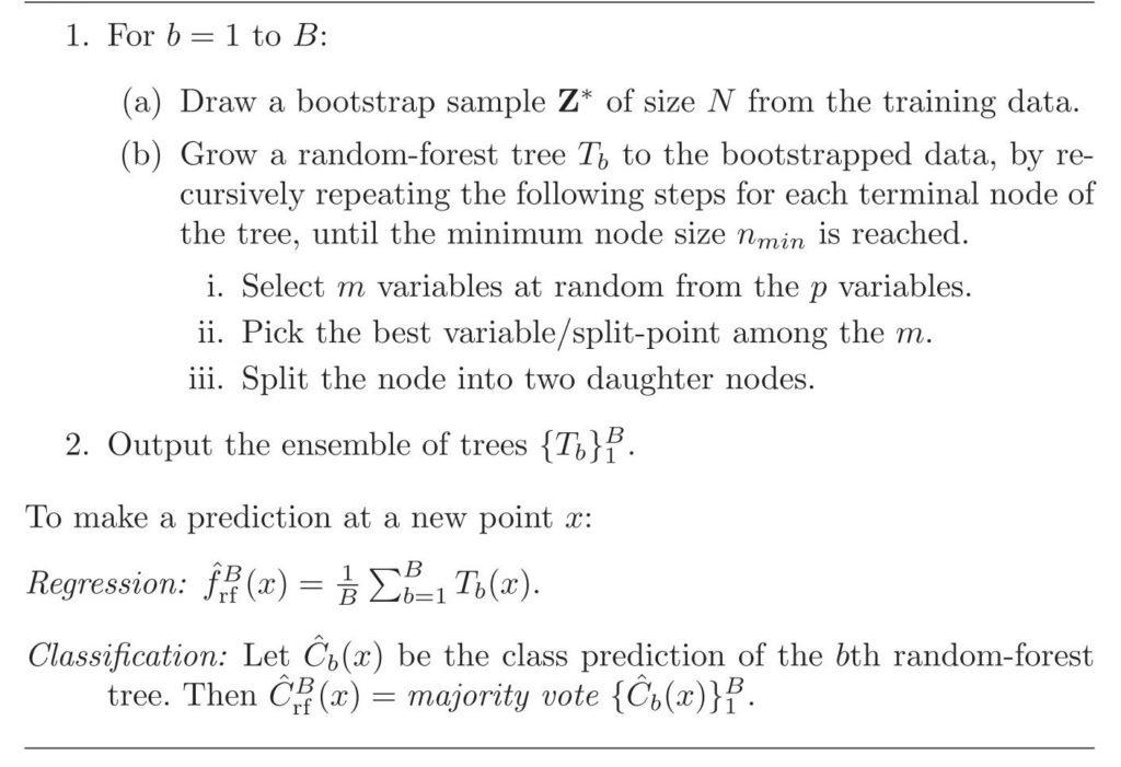
Concerning the choice of $p_{s}$ , for classification tasks $p_{s} \approx \sqrt{p}$ and a minimum node size of five is typical. In a regression setting, the default value for $p_{s} \approx \frac{p}{3}$ and the minimum node size is five.

But the values for $p_{s}$ should be considered as a tuning parameter, because its optimal value depends on the respective problem in question. Concerning a data set with a low number of relevant variables and a high number of attributes in general RF combined with a low $p_{s}$ , the algorithm performs quite poorly, because the probability of picking a relevant variable for a given split is quite low. So, in these settings, the choice of $p_{s}$ should be done very carefully.

Regarding the advantages of RF, it is possible to state that the method performs very well on large dataset without the need of further data preparation obtaining competitive results. But on the other hand, RF are not easy to interpret and they suffer of overfitting when being confronted with noisy classification or regression. In addition to that, the computational cost of a RF setting can be very high depending on the hyperparameter chosen for the model.

Boosting

Within the dependent ensemble methods, the most popular representative is the so-called boosting. The method draws its strengths like bagging from the fact of using multiple model for the prediction. But the methods are fundamentally different.

In boosting, instead of fitting distinct models to the respective bootstrapped samples in parallel, the main idea behind boosting is to grow an ensemble incrementally by adding each model at a time using an updated version of the original data set. One of the first boosting algorithms, the Adaboost or Adaptive boost for binary classification tasks, illustrates the functioning of the boosting process quite well (see Figure 6).

Given the above mentioned dataset with input features X and target variable Y, a weight distribution $D_{t}$ corresponding to the training data points with $D_{1}(i)=\frac{1}{m} \,\, for \, \, i=1,2,…,m$ is initialized. Then a loop from t=1 to T is initialized. Within the loop, first of all, a weak learner (e.g. a decision tree stump) minimizing the error and showing an accuracy of at least 0.5 is induced. This learner outputs a hypothesis for every observation i either 1 or -1. Comparing the results of the learner with the real target values, an error rate of $\epsilon_{t}$ can be calculated for the respective model. By evaluating the error rate of an individual model, its contribution $\alpha$ to the performance of the integral ensemble model can be determined. If the $\alpha_{t}$ is high, in other words if the error rate of the respective model is low, the contribution of the individual model to the integral ensemble model is high. Otherwise if the $\alpha_{t}$ of the model is low (or put it differently, if the error rate is high) the contribution of the individual model is low.

After having determined $\alpha_{t}$ , the weights of the respective data points of the training set are updated. The idea is to change the weights sequentially after each individual model added to get the next model to focus on the data points which the previously generated models misclassified:

The weight distribution $D_{t+1}$ is updated and each observation weight $D_{t}(i)$ is multiplied by the term $e^{(-\alpha * y * h(x_{i}))}$ Proceeding that way, the term is negative if $y_{i}=h(x_{i})$ and the value of $e^{-\alpha}$ can easily be calculated. On the other hand, if $y_{i} \neq h(x_{i})$ or in other words the model misclassified the observation in question, the value of $e^{\alpha}$ is calculated in the same manner.

Given an $\alpha$ obviously, the weights of the observations which have been classified correctly will decrease and those having been misclassified will increase.

The loop iterates T times obtaining T individual models, which are then combined in the last step by:

H(x)=sig(\sum_{t=1}^{T} \alpha_{t} * h_{t})

outputting a final prediction weighting every weak learner according to its individual performance.If the term within the signum function is equal or greater than 0, the final prediction is +1 and otherwise the final prediction is -1.

The concept of boosting should now be clear and Figure 7 subsumes again the differences and particularities of bagging and boosting.

Beside the adaptive boosting mentioned above, there exist another popular way of boosting: Gradient Boosting. The aim of this method is to use the gradient of the loss-function to fit a model step-wise, in small boosts, to the underlying data. Another article will introduce this popular concept further.

Sources

Breiman, Leo (2001): Random Forests. In: Machine Learning 45, S. 5–32.
Dietterich, Thomas G. (2000): Ensemble Methods in Machine Learning. In: Gerhard Goos, Juris Hartmanis und Jan Leeuwen (Hg.): Multiple Classifier Systems. First International Workshop, MCS 2000 Cagliari, Italy, June 21-23, 2000 Proceedings. Berlin, Heidelberg: Springer (Lecture Notes in Computer Science, 1857), S. 1–15.
Freund, Yoav; Schapire, Robert E. (1996): Experiments with a New Boosting Algorithm. In: Lorenza Saitta (Hg.): Machine learning. Proceedings of the thirteenth international conference, Bari, Italy, July 3 – 6, 1996. San Francisco, Calif.: Kaufmann, S. 148–156.
Freund, Yoav; Schapire, Robert E. (1999): A Short Introduction to Boosting. In: Journal of Japanese Society for Artificial Intelligence 14 (5), S. 771–780.
Hastie, Trevor; Tibshirani, Robert; Friedman, Jerome H. (2017): The elements of statistical learning. Data mining, inference, and prediction. Second edition, corrected at 12th printing 2017. New York, NY: Springer (Springer series in statistics).
James, Gareth; Witten, Daniela; Hastie, Trevor; Tibshirani, Robert (2017): An introduction to statistical learning. With applications in R. Corrected at 8th printing. New York, Heidelberg, Dordrecht, London: Springer (Springer texts in statistics).
Khandelwal, Renu (2018): Decision Tree and Random Forest. Hg. v. medium.com. Online verfügbar unter https://medium.com/datadriveninvestor/decision-tree-and-random-forest-e174686dd9eb.
Kuncheva, Ludmila I. (2014): Combining Pattern Classifiers. Methods and Algorithms. 2. Aufl. s.l.: Wiley.
Nisbet, Robert; Elder, John F.; Miner, Gary (2009): Handbook of statistical analysis and data mining applications. Amsterdam, Boston: Academic Press/Elsevier.
Rokach, Lior (2010): Ensemble-based classifiers. In: Artificial Intelligence Review 33 (1-2), S. 1–39. DOI: 10.1007/s10462-009-9124-7.
Schapire, Robert E. (1990): The strength of weak learnability. In: Machine Learning 5, S. 197–227.
Schapire, Robert E. (2013): Explaining AdaBoost. In: Bernhard Schölkopf, Zhiyuan Luo und Vladimir Vovk (Hg.): Empirical Inference. Festschrift in Honor of Vladimir N. Vapnik. Berlin, Heidelberg, s.l.: Springer Berlin Heidelberg, S. 37–52.

Ensemble Learning